2. Monte-Carlo Sampling and Importance Sampling
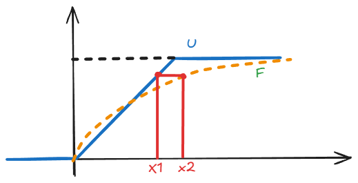
Monte-Carlo estimates an expectation by averaging samples, while importance sampling reweights samples from a proposal distribution to cut the variance. Use them when the integral has no closed form, and as the sampling intuition behind MCMC and variational methods.
- Reading time
- 4 min
- Length
- 676 words
- Updated
- Sep 15, 2026
- Total views
- --
1. Basic Concepts
(1) Sampling Preliminaries
1) Distribution transformation
In the sampling functions, we call (0, 1) and then transform it by some distribution function.
To sample in numpy, we can use rng = np.random.default_rng and then use rng.uniform to sample a uniform distribution. We set
Then we use an exponential distribution with parameter
the cumulative distribution function would be :
in order to transform a
Since
here
As a general case, the following part gives the transform from a normal distribution to a exponential distribution :
import numpy as np
import matplotlib.pyplot as plt
from scipy.stats import norm

# Number of samples
n_samples = 10_000

# Create a random number generator
rng = np.random.default_rng(seed=42)

# Step 1: Sample U from the uniform distribution (0, 1)
u = rng.normal(0.0, 1.0, size=n_samples)

# Step 2: Transform U into an exponential random variable
lam = 1.0  # Exponential distribution rate parameter
x = -np.log(1.0 - norm.cdf(u)) / lam

# Step 3: Plot the samples as a bar-style histogram
x_max = np.percentile(x, 99)  # Avoid displaying extreme outliers
bins = np.linspace(0, x_max, 40)
# Theoretical exponential probability density function
x_theory = np.linspace(0, x_max, 500)
pdf = lam * np.exp(-lam * x_theory)

plt.hist(
    x,
    bins=bins,
    density=True,
    alpha=0.75,
    color="steelblue",
    edgecolor="black",
    label="Generated samples"
)
plt.plot(
    x_theory,
    pdf,
    color="red",
    linewidth=2,
    label=r"Theoretical PDF: $\lambda e^{-\lambda x}$"
)

plt.xlabel("x")
plt.ylabel("Probability density")
plt.title("Sampling an Exponential Distribution by Inverse CDF")
plt.legend()
plt.tight_layout()
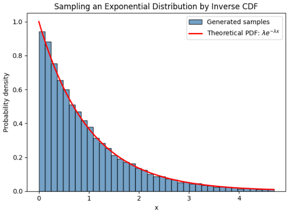
plt.show()Which can yield the distribution graph as follows :
2) Reliability Analysis & Monte Carlo sampling
Firstly, to define whether a structure is safe or failure, we use a performance function :
And we define the failure region as
where
We note since we already use
The variance of the failure probability can be calculated as :
The coefficient of variation (CoV) of the Monte Carlo estimator is :
(2) Importance sampling
1) Computation of Failure probability
We know in the Monte-Carlo sampling method, we define the performance function
where
However, we can still use another sampling function
This is called Importace sampling[1][2]
2) Mean, standard deviation, and coefficient of variation
Define the importance weight and the contribution of sample
The importance-sampling estimator is
Thus, the estimator is unbiased. Its variance (theoretical variance) is :
Therefore, the standard deviation (standard error) is :
For a simulation estimate, let
We also note in (1.2.8), the term of
Finally, for
and its practical estimate is
A good importance density
3) Optimal Importance sampling function
In the structural reliability analysis, we often sample near the failure point, we define as the "design point", which is
In practical case, we often use the normal distribution near the design point, i.e.,
Reference
吕震宙, 宋述芳, 李璐伟等, 结构/机构可靠性设计基础 [M] 西北工业大学出版社, 2019.3 ↩︎