4. Markov-decision-process

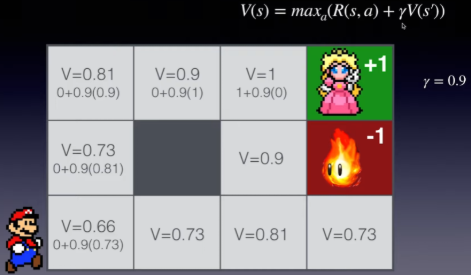
A Markov decision process formalizes sequential decision making with states, actions, rewards and transition probabilities. Use it to set up value and policy iteration, and as the base model that reinforcement learning methods optimize.

Reading time

9 min

Length

1,705 words

Updated

Sep 15, 2026

Total views

--

#math/counting-measure#math/markov-decision-process#math/optimization-policy#math/Reinforcement-learning/Bellman-equation

1. Preliminaries

(1) Counting Measure

We define the Counting Measure^[1] in mathematics, the counting measure can be defined on any measurable space (for example, the set $X$ on any Sigma-algebra, see Definition. sigma-algebra^[2]), but it's often in a countable sets.

In combinatorics theory, we denote the ground set as $X$, then the ==sigma-algebra== $\mathrm{\Sigma }$ defined by such ground set $X$ is given by :

$$\begin{array}{}\text{(1.1.1)}& \mathrm{\Sigma }\subset \mathbb{P}(X)\end{array}$$

Where $\mathbb{P}(X)$, or $2^X$ means the power set of $X$^[3] (to be more clean, all of the subsets).

After that, the $(X,\mathrm{\Sigma })$ forms a positive measure space $\mathrm{\Sigma }\to [0,+\mathrm{\infty }]$. Then the counting measure is only $\sigma$-finite if and only if the space $X$ is countable.

Then, the counting measure is the positive measure $\mathrm{\Sigma }\to [0,+\mathrm{\infty }]$, defined by :

$$\begin{array}{}\text{(1.1.2)}& \mu (A)=\{\begin{array}{l}|A|\text{if}A\text{ is a finite set}\\ +\mathrm{\infty }\text{if}A\text{ is an infinite set}\end{array}\end{array}$$

for all $A\in \mathrm{\Sigma }$, where $|A|$ is the cardinality(number of elements) of set $A$.

Notations We often use $(X,\mathrm{\Sigma },\mu )$ to denote a space. For this part, the first parameter is ground set, second is its subsets. Third (optional) is the measure.

(2) Integration on the counting measure

1. Discrete representation

We take the measure space $(\mathbb{N},2^{\mathbb{N}},\mu )$, Take any measurable function $f:\mathbb{N}\to [0,+\mathrm{\infty }]$. it can be ==represented pointwise== as follows :

$$\begin{array}{}\text{(1.2.1)}& f(x)=f(1)+f(2)+\dots f(n)+\cdots +f(\mathrm{\infty })\end{array}$$

then we got :

$$\begin{array}{}\text{(1.2.2)}& f(x)=\sum _{n=1}^{\mathrm{\infty }}f(n)1_{\{n\}}(x)=\underset{M\to \mathrm{\infty }}{lim}\underset{{\varphi }_M(x)}{\underbrace{\sum _{n=1}^{M}f(n)1_{\{n\}}(x)}}\end{array}$$

where we represent the $1_{\{n\}}$ as :

$$\begin{array}{}\text{(1.2.3)}& {\mathbf{1}}_{\{n\}}(x)=\{\begin{array}{ll}1& \text{x= n}\\ 0& \text{otherwise}\end{array}\end{array}$$

Here, $\{n\}$ means a singleton with element $n$, and each ${\varphi }_M$ is measurable. apparently, ${\varphi }_{M+1}(x)={\varphi }_M+f(M+1)\ge {\varphi }_M(x)$

2. Integration of function over countable measure

From (1.2.2), we know a function $f(x)$ can be represented with ${\varphi }_M(x)$, i.e., :

$$\begin{array}{}\text{(1.2.4)}& f(x)=\underset{M\to \mathrm{\infty }}{lim}{\varphi }_M(x){\varphi }_M(x)=\sum _{n=1}^{M}f(n){\mathbf{1}}_{\{n\}}(x)\end{array}$$

here, since $\mu$ is countable measure, we have $\mu (\{n\})=1$, so, for any measure $\mu$ on the space $(X,\mathrm{\Sigma },\mu )$ :

$$\begin{array}{}\text{(1.2.5)}& {\int }_{\mathbb{N}}{\varphi }_{M}d\mu =\sum _{n=1}^{M}f(n){\int }_N{\mathbf{1}}_{\{n\}}(x)d\mu =\sum _{n=1}^{M}f(n)\mu (\{n\})\end{array}$$

So we have the integral over the countable measure is :

$$\begin{array}{}\text{(1.2.6)}& \boxed{{\displaystyle {\int }_{\mathbb{N}}f(x)d\mu =\sum _{n=1}^{\mathrm{\infty }}f(n)}}\end{array}$$

We note that, this integration also defines a measure $\tilde{\mu }$ on $(X,\mathrm{\Sigma })$ via :

$$\begin{array}{}\text{(1.2.7)}& \tilde{\mu }(A):=\sum _{a\in A}f(a)\mathrm{\forall }A\in X\end{array}$$

the $\tilde{\mu }$ is a new measure on $A$, with taking $f(x)=1$ gives counting measure.

(3) Concepts in the random, probabilistic process and RL

These concepts can be found in ^[4]

STATE : a numeric representation of what the agent is observing at a particular point of time in the environment ACTION : the input the agent provides to the environments, calculated by applying a policy to the current state REWARD : feedback signal from the environment reflecting how well the agent is performing the goals.

The goal is for the current state, choose optimal action to maximize the long-term expected reward provided by the environment.

Such conceptions is also very basic in the control systems, this is. Current State + Action determines the new state ^[5]

2. Markov-decision-process (MDP)

(1) Definition of MDP

The reinforced learning is a model for a system evolves as different actions applied to the system. For a Markov decision process (MDP)^[6][7], that defined by the following 4-element tuple :

$$\begin{array}{}\text{(2.1.1)}& \boxed{{\displaystyle \text{MDP: }(\mathcal{S},\mathcal{A},P_a,R_a)}}\end{array}$$

This means : available state, available action, model decision and reward

We describe the Markov decision process as a 4-tuple process where :

1. $\mathcal{S}$ is a set of states called state space
2. $\mathcal{A}$ is a set of actions called action space, and $A_s$ often refers to the set of actions available from state $\mathcal{S}$.
3. $P_a$ is a intuitive level, or called $P_a(s,s^{\prime })$. For the action $a$ in state $s$ will lead to $s^{\prime }$ at the time $t+1$. This is defined to satisfy following relation :

$$\begin{array}{}\text{(2.1.2)}& \text{Pr}(s_{t+1}\in S^{\prime }|s_t=s,a_t=a)\stackrel{\text{action determined}}{⟶}{\int }_{S^{\prime }}{P}_a(s,s^{\prime })d{s}^{\prime }\end{array}$$

$\text{Pr}$ describes the ==probability that what probability the next state to reach, under certain state and actions==. This is integral for every $S^{\prime }\subset S$ measurable. 4. $R_a$ is immediate reward, or expected immediate reward received after action $a$ is taken. and such reward is a general random variable.

$P_a(s,s^{\prime })$ is the transition of the system $R_a(s,s^{\prime })$ often is $1$ when the state after transition is correct.

(2) Simple example

A simple example is the robot navigation system (source: ^[8]):

robotics navigation system

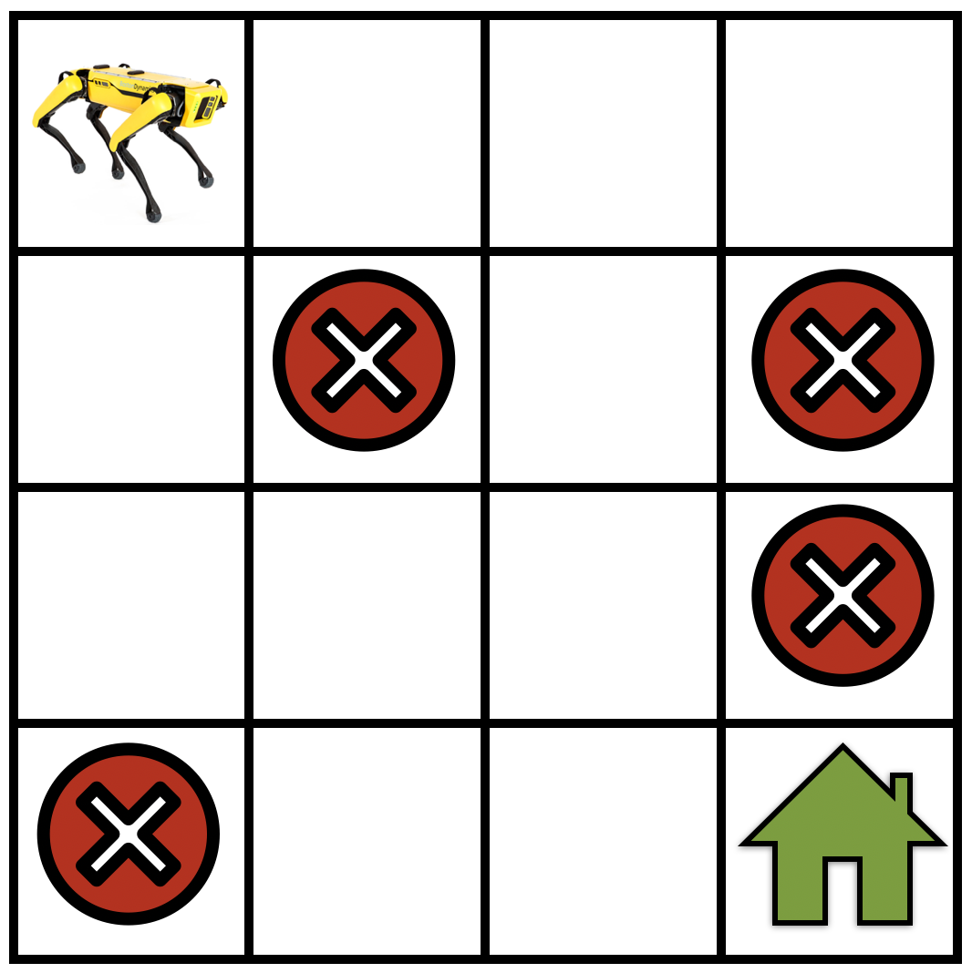
For the above robotics navigation task shown in Fig. 2.1, we have :

1. $\mathcal{S}$ is the set of states in the MDP, as the navigation gridworld shows.
2. $\mathcal{A}$ is the actions that robot can take at each state, e.g., “go forward”, “turn right”, “turn left”, “stay at the same location”.
3. If we don't know that the robot moves exactly but only up to some approximation, this amounts to defining a transition function that from current state $s$ to a new state $s^{\prime }$.

$$\begin{array}{}\text{(2.2.1)}& T:\mathcal{S}\times \mathcal{A}\times \mathcal{S}\to [0,1]\end{array}$$

such that it's condition probability (here for example $\text{forward}\to T=0.8$, $\text{turn right}\to T=0.1$, so we said $\to [0,1]$)

$$\begin{array}{}\text{(2.2.2)}& T(s,a,s^{\prime })=P(s^{\prime }|s,a)\end{array}$$

And the transition function is a probability distribution that $\sum _{s^{\prime }\in \mathcal{S}}T(s,a,s^{\prime })=1$ for all $s\in \mathcal{S}$ and $a\in \mathcal{A}$. So in many cases, like (2.1.1), we use $P$ instead of $T$ here.

We can construct a notion using the concept of reward $r:\mathcal{S}\times \mathcal{A}\to \mathbb{R}$, we can say that the robot gets a reward $r(s,a)$ if robot takes an action $a$ at state $s$. Such reward is designed by the user.

(3) Return Factor and Discount Factor

For the MDP in (2.1.1), the continues taking actions to result in a trajectory :

$$\begin{array}{}\text{(2.3.1)}& \tau =(s_0,a_0,r_0,s_1,a_1,r_1,\dots )\end{array}$$

For each time step $t$, the robot is at state $s_t$, then we define the return of the trajectory as :

$$\begin{array}{}\text{(2.3.2)}& R(\tau )=r_0+r_1+r_2+\dots \end{array}$$

The goal is to reach the final state that scores as fast as possible, if we scores at time $t$, the reward $R_a$. But if the wanted state is reached at $t+1$, we set the reward as $\gamma R_a$ , we also introduce the discount factor $\gamma$, which is often defined by the discount rate $r$ :

$$\begin{array}{}\text{(2.3.3)}& \gamma =\frac{1}{1+r}\end{array}$$

A lower discount factor makes the decision maker more short-sighted (greedy for recent best solutions). Then the discounted return, or "reward" here, such reward is defined as :

$$\begin{array}{}\text{(2.3.4)}& \boxed{{\displaystyle R(\tau )=\sum _{t=0}^{\mathrm{\infty }}{\gamma }^t{R}_{a_t}}}\end{array}$$

And for a large value of the discount factor, e.g. $\gamma =0.99$, then robot is encouraged to explore more and find the best trajectory. A successful value often between $\gamma \in [0.9,0.99]$

(4) Optimization Policy & Objective definition

The reinforcement learning problem is typically modeled using Markov Decision Processes. We consider that we want the reach a specific final goal. So we determine state of the result as $\pi (x)$ by a given policy. The objective as to maximize the cumulative function of the random rewards :

$$\begin{array}{}\text{(2.4.1)}& \eta (\pi )=\mathbb{E}[\sum _{t=0}^{\mathrm{\infty }}{\gamma }^t{R}_{a_t}(s_t,s_{t+1})]\end{array}$$

where $a_t=\pi (s_t)$, or Actions at each time step is defined given by the policy.

We note another objective function to use is the $H$, or the step return;

$$\begin{array}{}\text{(2.4.2)}& \mathbb{E}[\sum _{t=0}^{H-1}{R}_{a_t}(s_t,s_{t+1})]\end{array}$$

3. Bellman Optimality Equation

(1) For a determined-state problem

Firstly, we represent :

1. policy value function as $V_{\pi }(s)$
2. Optimal value function as $V^{\ast }(s)$ (We want to make policy function to approach this)

Bellman Equation^[9] helps evaluate the expected reward relative to the advantage or disadvantage of each state. the Value function is defined as :

$$\begin{array}{}\text{(3.1.1)}& \boxed{{\displaystyle V^{\ast }(s)=\underset{a}{max}[R(s)+\gamma V^{\ast }(s^{\prime })]}}\end{array}$$

here, $R$ is period-specific objective function, $V(s^{\prime })$ is the future objective function.

Sometimes, if $R$ is related with $a$ we use :

$$V^{\ast }(s)=\underset{a}{max}[R(s,a)+\gamma V^{\ast }(s^{\prime })]$$

Bellman showed that a dynamic optimization problem in discrete time can be stated in a recursive, step-by-step form known as backward induction by writing down the relationship between the value function in one period and the value function in the next period.

Here, $\underset{a}{max}$ means the choice of the best possible action. This means, to choose the best possible action, the value is the current response + weighted value of future possible states. For a more general equation, we still need to consider the probability of next option. i.e. adding $P(s^{\prime }|s)$ into (3.1.1) :

$$\begin{array}{}\text{(3.1.2)}& \boxed{{\displaystyle V(s)=\underset{a}{max}|R(s)+\gamma \sum _{s}P(s^{\prime }|s,a)V(s^{\prime })|}}\end{array}$$

We note in application case, we use (3.1.1) more than (3.1.2)

The often the ideal action is to take the reward from the end state back to the start, which means, the end state has been defined (as $\pi$ later). A comprehensive picture is drawn as follows (the $V$ is calculated by ):

The action is to bring us to the highest value function. So it's very easy to find the clean path.

(2) For A stochastic system

For example, a consumer with initial wealth endowment $s_0$, he also have instantaneous utility function $u(c)$ (this will determine the objective depends by the consumption, so this is deemed as "reward"), discounts the next period utility at a rate of $\beta$, and $c$ here denotes the consumption. We should choose a consumption plan, then the current interest rate on the left money in the bank is $r$.

So the consumer should choose a sequence $\{c_t\}$  such a way that their lifetime expected utility is maximized, so we often use following function :

$$\begin{array}{}\text{(3.2.1)}& \underset{\{c_t{\}}_{t=0}^{\mathrm{\infty }}}{max}\sum _{t=0}^{\mathrm{\infty }}{\beta }^{t}u(c_t)\end{array}$$

Then the constraint is :

$$\begin{array}{}\text{(3.2.2)}& s_{t+1}=(1+r)(s_t-c_t)c_t>0\underset{t\to \mathrm{\infty }}{lim}{a}_t\ge 0\end{array}$$

the value function should be :

$$\begin{array}{}\text{(3.2.3)}& V(s)=\underset{0\le c\le a}{max}\{u(c)+\beta V((1+r)(s_t-c))\}\end{array}$$

References

---

1. https://en.wikipedia.org/wiki/Counting_measure ↩︎

2. 1. Sigma-algebra and Lebesgue measure ↩︎

3. https://en.wikipedia.org/wiki/Power_set ↩︎

4. https://www.youtube.com/watch?v=14BfO5lMiuk ↩︎

5. https://en.wikipedia.org/wiki/Optimal_control ↩︎

6. https://en.wikipedia.org/wiki/Markov_decision_process ↩︎

7. https://d2l.ai/chapter_reinforcement-learning/mdp.html ↩︎

8. https://d2l.ai/chapter_reinforcement-learning/mdp.html ↩︎

9. https://en.wikipedia.org/wiki/Bellman_equation ↩︎