2. Strong and Weak Form of Linear Elasticity Equivalence

#mechanics/Cauchy-stress#mechanics/hooks-law#mechanics/linear-elasticity

The weak formulation of elasticity is fundamental to the finite-element analysis of ordinary, lattice, and homogenized structures. The weak form is also the basic for implementing the form in the FEniCSx

(1) Kinematics and constitutive equation

Let $\mathrm{\Omega }\subset {\mathbb{R}}^d$, with $d=2$ or $3$, be the reference domain, and let $u:\mathrm{\Omega }\to {\mathbb{R}}^d$ be the displacement field. A material point initially at $x$ moves to $x+u(x)$, so the deformation gradient is

$$\begin{array}{}\text{(1.1)}& F=\frac{\partial u_{new}}{\partial x}=I+\mathrm{\nabla }u.\end{array}$$

The Green--Lagrange strain is

$$\begin{array}{}\text{(1.2)}& E(u)=\frac{1}{2}(F^{T}F-I)=\frac{1}{2}(\mathrm{\nabla }u+\mathrm{\nabla }{u}^T+\mathrm{\nabla }{u}^T\mathrm{\nabla }u).\end{array}$$

Under the small-displacement-gradient assumption, the quadratic term is neglected. This gives the linearized strain tensor

$$\begin{array}{}\text{(1.3)}& \epsilon (u)=\frac{1}{2}(\mathrm{\nabla }u+\mathrm{\nabla }{u}^T)=\mathrm{sym}(\mathrm{\nabla }u).\end{array}$$

The linear constitutive equation is :

$$\begin{array}{}\text{(1.4)}& \sigma (u)=\mathbb{C}:\epsilon (u),{\sigma }_{ij}=C_{ijkl}{\epsilon }_{kl}(u),\end{array}$$

where $\sigma$ is the Cauchy stress and $\mathbb{C}$ is the fourth-order stiffness tensor, with units of Pa. Its inverse, when it exists, is the compliance tensor and has units of ${\text{Pa}}^{-1}$.^[1]

For an isotropic material,

$$\begin{array}{}\text{(1.5)}& \mathbb{C}:\xi =2\mu \xi +\lambda \mathrm{tr}(\xi )I,\end{array}$$

and therefore

$$\begin{array}{}\text{(1.6)}& \sigma (u)=2\mu \epsilon (u)+\lambda \mathrm{tr}(\epsilon (u))I.\end{array}$$

For classical linear elasticity, We know that a stiffness tensor for general material has both minor symmetries major symmetry^[2]:

$$\begin{array}{}\text{(1.7)}& C_{ijkl}=C_{jikl}=C_{ijlk}=C_{klij}.\end{array}$$

(2) Strong form of Linear Elasticity

Split the boundary into a displacement boundary ${\mathrm{\Gamma }}_D$ and a traction boundary ${\mathrm{\Gamma }}_N$:

$$\begin{array}{}\text{(2.1)}& \partial \mathrm{\Omega }=\overline{{\mathrm{\Gamma }}_D\cup {\mathrm{\Gamma }}_N},{\mathrm{\Gamma }}_D\cap {\mathrm{\Gamma }}_N=\varnothing .\end{array}$$

Let $n$ be the outward unit normal, $f$ the body-force density, $u_D$ the prescribed displacement, and $g$ the prescribed traction. Static balance of linear momentum is

$$\begin{array}{}\text{(2.2)}& \boxed{{\displaystyle -\mathrm{\nabla }\cdot \sigma =f\text{in }\mathrm{\Omega },}}\end{array}$$

where, in index notation,

$$\begin{array}{}\text{(2.3)}& -(\mathrm{\nabla }\cdot \sigma {)}_i=-\frac{\partial {\sigma }_{ij}}{\partial x_j}=f_i.\end{array}$$

Strong form of linear elasticity Find $u$ such that

$$\begin{array}{}\text{(strong-form-of-linear-elasticity)}& \{\begin{array}{ll}-\mathrm{\nabla }\cdot (\mathbb{C}:\epsilon (u))=f& \text{in }\mathrm{\Omega },\\ u=u_D& \text{on }{\mathrm{\Gamma }}_D,\\ (\mathbb{C}:\epsilon (u))n=g& \text{on }{\mathrm{\Gamma }}_N.\end{array}\end{array}$$

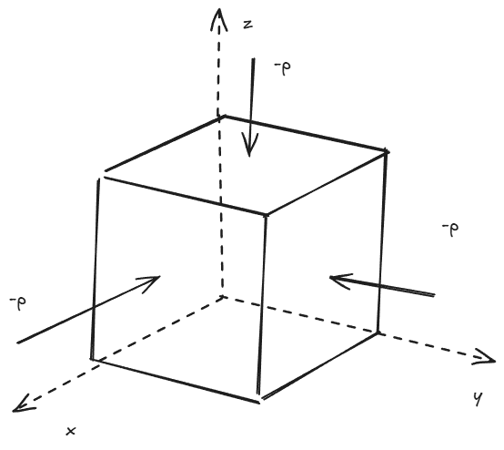
Where $g$ is the traction applied on the pressure boundaries.

The homogeneous displacement condition used in many examples is the special case $u_D=0$. TopCut,^[3] for example, uses the same equilibrium equation with $f=0$.

(3) Derivation of the weak form

The unknown $u$ is the trial function. Let $v$ be an arbitrary test function that vanishes on the displacement boundary:

$$\begin{array}{}\text{(3.1)}& v=0\text{on }{\mathrm{\Gamma }}_D.\end{array}$$

Multiply the equilibrium equation by $v$ and integrate over $\mathrm{\Omega }$:

$$\begin{array}{}\text{(3.2)}& {\int }_{\mathrm{\Omega }}-(\mathrm{\nabla }\cdot \sigma )\cdot vd\mathrm{\Omega }={\int }_{\mathrm{\Omega }}f\cdot vd\mathrm{\Omega }.\end{array}$$

Integration by parts (the divergence theorem) gives :

$$\begin{array}{}\text{(3.3)}& {\int }_{\mathrm{\Omega }}-(\mathrm{\nabla }\cdot \sigma )\cdot vd\mathrm{\Omega }={\int }_{\mathrm{\Omega }}\sigma :\mathrm{\nabla }vd\mathrm{\Omega }-{\int }_{\partial \mathrm{\Omega }}(\sigma n)\cdot vd\mathrm{\Gamma }.\end{array}$$

This follows component-wise from:

$$\begin{array}{}\text{(3.4)}& \frac{\partial }{\partial x_j}({\sigma }_{ij}{v}_i)=\frac{\partial {\sigma }_{ij}}{\partial x_j}{v}_i+{\sigma }_{ij}\frac{\partial v_i}{\partial x_j}.\end{array}$$

Because $\sigma$ is symmetric, it is orthogonal to the skew-symmetric part of $\mathrm{\nabla }v$. Hence

$$\begin{array}{}\text{(3.5)}& \sigma :\mathrm{\nabla }v=\sigma :\epsilon (v).\end{array}$$

The boundary term splits over ${\mathrm{\Gamma }}_D$ and ${\mathrm{\Gamma }}_N$. On ${\mathrm{\Gamma }}_D$, $v=0$; on ${\mathrm{\Gamma }}_N$, $\sigma n=g$. Consequently,

$$\begin{array}{}\text{(3.6)}& {\int }_{\mathrm{\Omega }}\sigma (u):\epsilon (v)d\mathrm{\Omega }={\int }_{\mathrm{\Omega }}f\cdot vd\mathrm{\Omega }+{\int }_{{\mathrm{\Gamma }}_N}g\cdot vd\mathrm{\Gamma }.\end{array}$$

Substituting $\sigma (u)=\mathbb{C}:\epsilon (u)$ yields the weak equation

$$\begin{array}{}\text{(3.7)}& \boxed{{\displaystyle {\int }_{\mathrm{\Omega }}\epsilon (v):\mathbb{C}:\epsilon (u)d\mathrm{\Omega }={\int }_{\mathrm{\Omega }}f\cdot vd\mathrm{\Omega }+{\int }_{{\mathrm{\Gamma }}_N}g\cdot vd\mathrm{\Gamma }.}}\end{array}$$

(4) Function spaces and weak problem

The trial and test spaces are different when the prescribed displacement is nonzero:

$$\begin{array}{}\text{(4.1)}& U=\{u\in [H^1(\mathrm{\Omega }){]}^d:u{|}_{{\mathrm{\Gamma }}_D}=u_D\},\end{array}$$

$$\begin{array}{}\text{(4.2)}& V=\{v\in [H^1(\mathrm{\Omega }){]}^d:v{|}_{{\mathrm{\Gamma }}_D}=0\}.\end{array}$$

If $u_D=0$, then $U=V$. The requirement $v=0$ applies only on ${\mathrm{\Gamma }}_D$, not on the entire boundary; otherwise the applied traction on ${\mathrm{\Gamma }}_N$ would disappear from the formulation.

[!theorem] Weak form of linear elasticity Find $u\in U$ such that, for every $v\in V$,

$$\begin{array}{}\text{(weak-form-of-linear-elasticity)}& \boxed{{\displaystyle {\int }_{\mathrm{\Omega }}\epsilon (v):\mathbb{C}:\epsilon (u)d\mathrm{\Omega }={\int }_{\mathrm{\Omega }}f\cdot vd\mathrm{\Omega }+{\int }_{{\mathrm{\Gamma }}_N}g\cdot vd\mathrm{\Gamma }}}.\end{array}$$

Equivalently, define

$$\begin{array}{}\text{(4.3)}& a(u,v)={\int }_{\mathrm{\Omega }}\epsilon (v):\mathbb{C}:\epsilon (u)d\mathrm{\Omega },\end{array}$$

and

$$\begin{array}{}\text{(4.4)}& \ell (v)={\int }_{\mathrm{\Omega }}f\cdot vd\mathrm{\Omega }+{\int }_{{\mathrm{\Gamma }}_N}g\cdot vd\mathrm{\Gamma }.\end{array}$$

Then the problem is simply

$$\begin{array}{}\text{(4.5)}& a(u,v)=\ell (v)\text{for every }v\in V.\end{array}$$

(5) Index notation and simplification

Equation $\text{(4.3)}$ can be written as

$$\begin{array}{}\text{(5.1)}& {\int }_{\mathrm{\Omega }}{C}_{ijkl}{\epsilon }_{kl}(u){\epsilon }_{ij}(v)d\mathrm{\Omega }={\int }_{\mathrm{\Omega }}{f}_i{v}_{i}d\mathrm{\Omega }+{\int }_{{\mathrm{\Gamma }}_N}{g}_i{v}_{i}d\mathrm{\Gamma }.\end{array}$$

Using

$$\begin{array}{}\text{(5.2)}& {\epsilon }_{kl}(u)=\frac{1}{2}(\frac{\partial u_k}{\partial x_l}+\frac{\partial u_l}{\partial x_k}),\end{array}$$

and the minor symmetry $C_{ijkl}=C_{ijlk}$,

$$\begin{array}{}\text{(5.3)}& \begin{array}{rl}{C}_{ijkl}{\epsilon }_{kl}(u)& =\frac{1}{2}{C}_{ijkl}\frac{\partial u_k}{\partial x_l}+\frac{1}{2}{C}_{ijkl}\frac{\partial u_l}{\partial x_k}\\ & =\frac{1}{2}{C}_{ijkl}\frac{\partial u_k}{\partial x_l}+\frac{1}{2}{C}_{ijlk}\frac{\partial u_k}{\partial x_l}\\ & =C_{ijkl}\frac{\partial u_k}{\partial x_l}.\end{array}\end{array}$$

Applying the other minor symmetry to the test-function gradient gives the equivalent expression

$$\begin{array}{}\text{(5.4)}& \boxed{{\displaystyle {\int }_{\mathrm{\Omega }}{C}_{ijkl}\frac{\partial u_k}{\partial x_l}\frac{\partial v_i}{\partial x_j}d\mathrm{\Omega }={\int }_{\mathrm{\Omega }}{f}_i{v}_{i}d\mathrm{\Omega }+{\int }_{{\mathrm{\Gamma }}_N}{g}_i{v}_{i}d\mathrm{\Gamma }}}.\end{array}$$

For a perforated or heterogeneous microscopic domain ${\mathrm{\Omega }}^{\epsilon }$, as commonly used for lattice structures and homogenization, replace $\mathrm{\Omega }$ by ${\mathrm{\Omega }}^{\epsilon }$ and use its corresponding boundary partition. The derivation is otherwise unchanged.

---

1. Constitutive equation ↩︎

2. 1. Symmetric Stiffness Tensor and Voigt notation ↩︎

3. Andreasen, Casper Schousboe, Martin Ohrt Elingaard, and Niels Aage. “Level Set Topology and Shape Optimization by Density Methods Using Cut Elements with Length Scale Control.” Structural and Multidisciplinary Optimization 62, no. 2 (2020): 685–707. https://doi.org/10.1007/s00158-020-02527-1. ↩︎